BH3, an Example of an MO
Computation
and an Apology for Local Bonds
Quantum mechanical calculations on smallish molecules are now
routine. Although most of our thinking in Chem 125 will be based on
more qualitative application of quantum mechanical ideas, it is useful
to see what the results of such a calculation look like as a check on
our qualitative approach to understanding bonds.
First one might consider the different goals of the various
approaches to determining electron distribution in molecules:
(1)
The
MOLECULE does not
have to deal with mathematics. It just does naturally what is
necessary to achieve its GOAL: to minimize the kinetic and
coulombic potential energy of its nuclei and electrons. This
results in a dynamic cloud of rapidly moving electrons within
which the slowly moving nuclei are embedded, rather like an
"inverted" plum-pudding atom of J.J. Thomson.
Various aspects of the nature of the molecule are accessible
from such experiments as:
X-ray diffraction, which measures electron density in
crystals,
IR spectroscopy, which measures differences between allowed
vibrational energy levels for motion of the nuclei,
ESR spectroscopy, which measures electron density at
magnetic nuclei (e.g. 13C) for an "odd" electron,
one whose magnetism is not cancelled by pairing with another
electron.
(2)
The
COMPUTER has a different
GOAL: to compute electron densities and molecular energy by
applying some approximate version of the Schrödinger equation in order to minimize the kinetic and
potential energy for the set of particles. Because the
equation is too complex to solve exactly, the computer makes
approximations that, hopefully, provide an acceptable compromise
between affordability and realism. Typical approximations include
holding the nuclei fixed while calculating the electronic wave
functions (Born-Oppenheimer approximation), treating a
many-electron wave function as a product of molecular orbitals,
approximating the molecular orbitals as weighted sums of a limited number
of atomic orbitals on different atoms, and approximating the
atomic orbitals by functions that are mathematically convenient
(this is the "basis set"). Programs can then correct approximately
for electron-electron repulsion using SCF. More sophisticated (and
computationally intensive) methods address the problem of dynamic
correlation.
Computational results may be used to predict, and can
be checked by, experiment. One can calculate the structure,
that is the nuclear arrangement that minimizes molecular
energy, or compare the energy of two different arrangements of
the same atoms (before and after reaction, for example).
Calculations also dissect the total electron density into
individual orbitals, which suggest one-electron
properties, such as the density at a magnetic nucleus (ESR), or
the energy required to move an electron from one orbital to
another (uv-visible light absorption), or to remove it from the molecule altogether (ionization potential).
(3) The STUDENT in Chemistry
125 has a different GOAL: to understand structure
and reactivity of organic molecules. Given the limitations of
the human mind, this requires finding the
simplest realistic model
for bonding. There is an unavoidable tension between
simplicity and realism. A model of atoms with little hooks
captures some of the features of bonding but it is obviously too
simple to be realistic.
The realism of the model can be judged by comparing
not only to experiment, but also to computation. We will not
demand the quantitative precision that the computer might
achieve, but the model must be quantum mechanically sound. To
be worthwhile it should take us well beyond where we can go
with the classical idea of lines for bonds. If it will
sometimes fail, we must be aware when to expect failure.
The point of this web page is to evaluate our model of
bonding by comparison with the results of a quantum mechanical
computation.
The following figures were generated by "MacSpartan", a typical
package that does very useful molecular orbital calculations at the
SCF level. But we made no attempt to estimate correlation energy. We
expect the computed electron density to be pretty faithful to nature,
but there will be a errors in energy (which we hope will mostly
cancel out when we do comparisons with computations for other
arrangements of the same atoms).
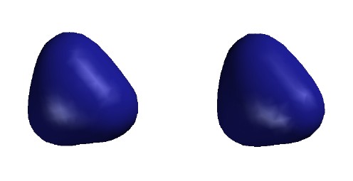
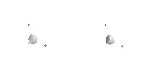
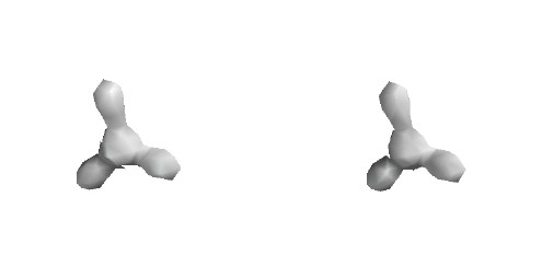
The first series of stereo-pair pictures shows different
visualizations of the TOTAL electron density of the planar
BH3 molecule. It represents the sum of the electron
densities calculated for the three occupied valence orbitals of this
molecule and for the 1s orbital on boron. Since this computation used
a reasonably large basis set of 21 atomic functions (called the
"6-31G*" basis set), this total electron density is probably a
very good approximation of what might be observed experimentally
by x-ray diffraction, if it were possible to grow a crystal of
BH3 molecules. This is of course an impossible experiment,
because, as we will discuss very soon, BH3 molecules react
in pairs to give B2H6. Note that the shape
depends significantly on which contour is shown.
|
|
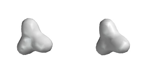
Total Electron Density
Note: these are stereo-pair
pictures that
may be viewed in three dimensions
Contour level 0.30
e/Ĺ3
Electron density higher near boron
than near hydrogen despite H's greater
valence-shell electronegativity. This is
probably due both to 1s core electrons and
to the 2s electron density within the radial node.
[Program not so good at drawing small
surfaces - fails to draw smooth shapes
and omits one H in error.]
|
|
|
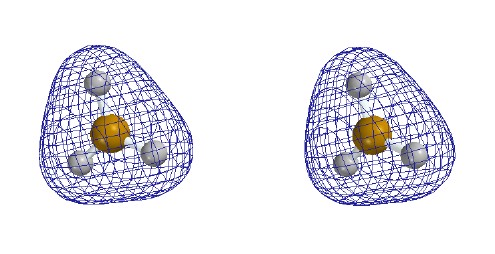
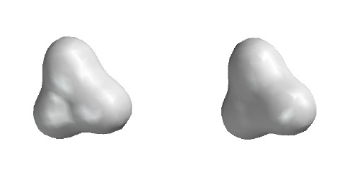
Total Electron Density
Contour level 0.15
e/Ĺ3
H density begins to "overtake" B density,
which is high near the nucleus, but falls
away quickly with increasing distance.
|
|
|
Total Electron Density
Contour level 0.05
e/Ĺ3
Note beginning of dimple near central B.
H density is dominant for the valence electrons.
|
|
|
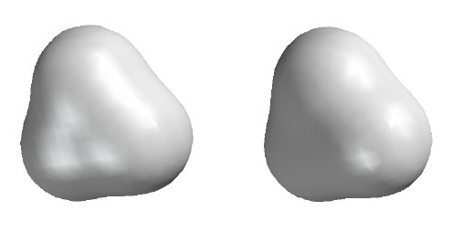
Total Electron Density
Contour level 0.02
e/Ĺ3
|
|
|
Total Electron Density
Contour level
0.002
e/Ĺ3
(This contour level approximates the "size"
of molecules. Adjacent molecules in solids
tend to be spaced such that their 0.002
surfaces touch. Thus this is a sort of
"van der Waals surface".)
|
|
|
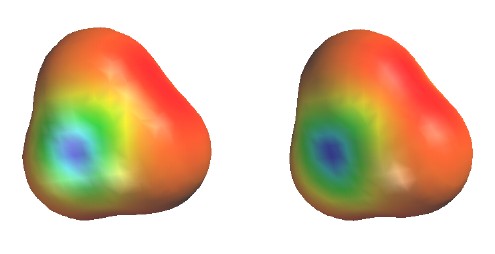
Total Electron Density
colored to show electrostatic
potential
Contour level
0.002
e/Ĺ3
(as in previous figure)
Colors show the energy of a test "proton"
at various positions on the surface.
Red shows low energy (negative region) near H;
Blue shows high energy (positive region) near B.
Uneven electron distribution due to poor energy match
of B-H bond (1s of H lower than 2sp2 hybrid of
B
|
|
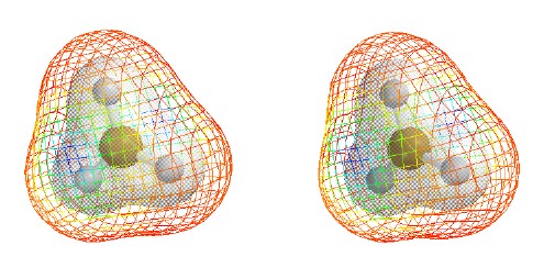
|
Total Electron Density
with electrostatic potential
Contour level
0.002
e/Ĺ3
(as in previous figure but drawn as mesh
to allow seeing 0.02 contour and the
ball and spoke model inside.)
|
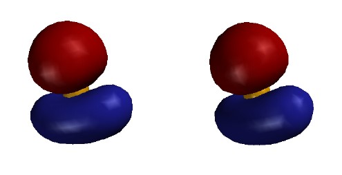
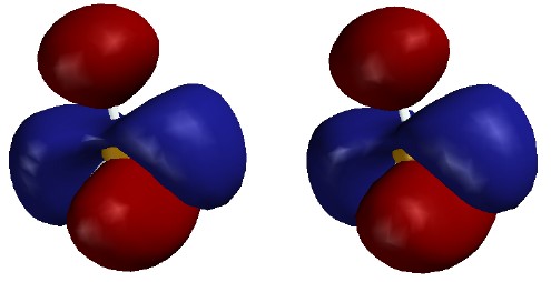
The following figures show how the computer parses the total
electron density into SCF molecular orbitals (presented in order of
increasing energy, omitting the lowest MO which is mostly the 1s core orbital on B). Since there are 7 valence-level atomic orbitals
(1s on each of three H atoms plus 2s and three 2p AOs on B) there are 7
orthogonal low-energy molecular orbitals that can be made from them. (Higher-energy MOs are constructed by mixing AOs with n > 2.) There are 6 valence electrons (i.e. three pairs: 3
electrons from B, 1 from each H), so only the first three of these
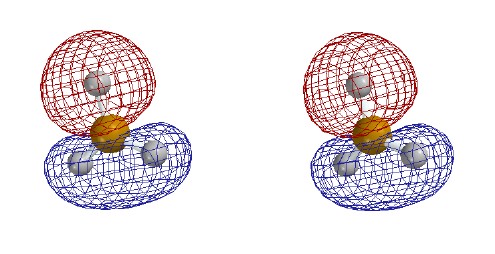
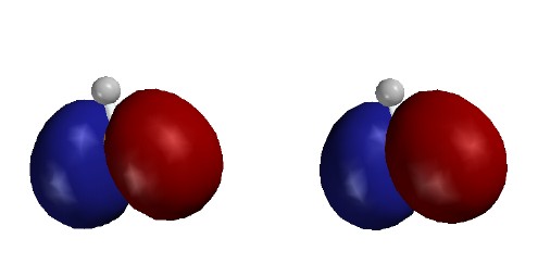
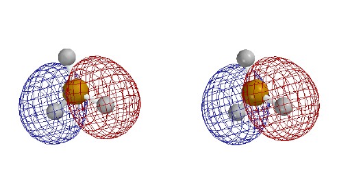
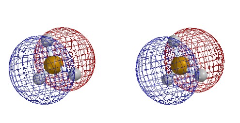
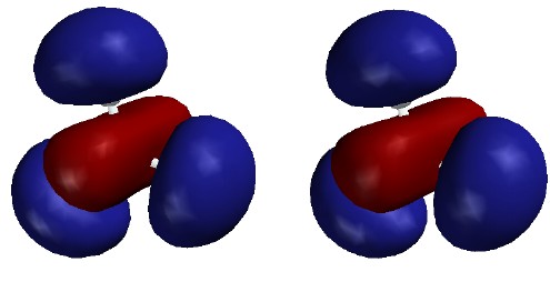
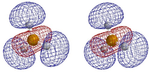
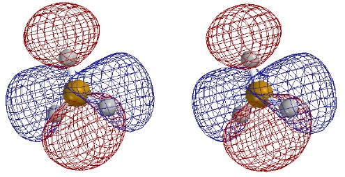
valence-level MOs are occupied. Each MO is shown as two stereo pairs. The pair on
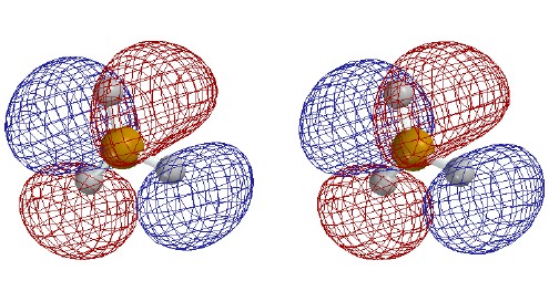
the left shows the contour at a given magnitude of psi colored red or
blue to denote the sign of the wave function. The pair on the right
shows the surface as a mesh to reveal the ball and spoke model.
Note that none of the three occupied MOs has a node between B and
H. All of them contribute to B-H bonding.
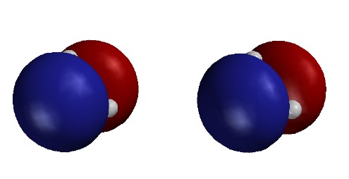
For simplicity of understanding we in Chem 125 will parse the
total electron density differently, into three localized and
equivalent B-H bonds, rather than into a lowest energy orbital
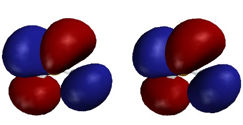
with no nodes (at the top) and two higher-energy orbitals with one
node each (the two immediately above). It is not surprising that
these two models predict the same overall total electron density and
energy, because the nodeless MO (the analogue of atomic 2s) can be viewed as the sum of the three
bonding orbitals; the first one-node MO (2px), as mostly the "vertical" B-H
bond minus a lesser amount of the sum of the "horizontal" B-H bonds;
and the second one-node MO (2py), as the difference between the "horizontal"
B-H bonds. Note that these MOs are bonding between B and H; their nodes pass through the B nucleus, not between B and H.
When the three localized B-H bonds are allowed by the computation to mix and form the delocalized MOs,
one MO combination (the one with no nodes) goes down in energy and the other two go up, but
the overall energy and electron density remains very nearly the
same. Furthermore, the individual MO energies don't shift very
much, because the B-H bond orbitals don't overlap well one another.
Typically bond orbitals overlap less than 10% as much as the hybrid
atomic orbitals whose overlap created the two bonds in the first
place, so the shifts are small.
Thus, especially for qualitative purposes, we are completely
justified in confining our attention to simpler localized bonding
orbitals, rather than coping with their combination into the more
complicated delocalized SCF MOs that the computer chooses. Since the
delocalized orbitals may be viewed as a combination of the localized
orbitals, the factors that influence the total energy of the
localized orbitals (for example distortion from a planar toward a
pyramidal structure) will influence the total energy of the
delocalized MOs in the same way.
This comparison with the "true" computational orbitals justifies our use of the simpler
local bond model.
When will our simplification into localized bonds fail?
(1) When (e.g. in the interaction with light) we are
interested in the individual energy, or the spatial distribution,
of a single pair of electrons, rather than the overall energy or total electron density.
(2) When (e.g. in the case of resonance) certain bonding orbitals
have strong overlap.
(3) When (e.g. in what we will call "pericyclic" reactions) we are interested in
multiple contacts between individual molecules that might lead to
reactivity at more than one position.
In such cases mixing of the localized bonding orbitals can indeed make a
difference, and we shall have to use a more sophisticated MO
model.
The 4th MO, the LUMO of BH3, is in fact an atomic 2p
orbital of B. It is like the 2p SOMO that is half-occupied by the
seventh electron in the analogous CH3 radical.
Note that the last three (highest energy) UMOs have nodes between
B and H. This is especially clear in the 5th MO (the 3s), which looks like a
red cylinder among three blue balls. These MOs are combination of
localized B-H antibonds in the same way that the lowest three MOs are
combinations of B-H bonds.
©copyright
2003,2008 J.M.McBride